Trajectories of Brownian motion

# Clear the workspace
rm(list = ls())

# Load required libraries
library(berryFunctions)
library(ggplot2)
library(gridExtra)

# Function to simulate Brownian Motion
sim.bm <- function(x, n_path = n_path) {
  tau <- x[1]
  bm <- cumsum(c(0, tau * rnorm(n_path - 1)))
  return(bm)
}

##### Simulation Parameters #####

n_path <- 100   # Number of time steps
start <- 1:(n_path - 1)
end <- 2:n_path
reps <- 100     # Number of repetitions

##### Simulation for sigma=1 #####

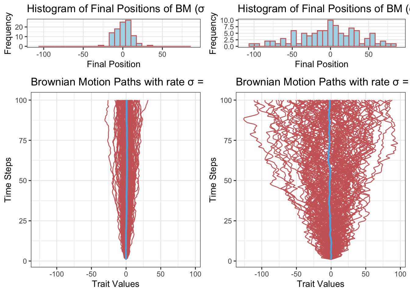
sigma1 <- 1
x1 <- c(sigma1)
sim.bm.array1 <- array(NA, c(reps, n_path))
for (i in 1:reps) {
  sim.bm.array1[i, ] <- sim.bm(x1, n_path = n_path)
}

##### Simulation for sigma=4 #####

sigma2 <- 4
x2 <- c(sigma2)
sim.bm.array2 <- array(NA, c(reps, n_path))
for (i in 1:reps) {
  sim.bm.array2[i, ] <- sim.bm(x2, n_path = n_path)
}

##### Plotting Brownian Motion Paths for sigma=1 #####

p1 <- ggplot() + 
  ylim(range(unlist(sim.bm.array1), unlist(sim.bm.array2))) +
  ggtitle("Brownian Motion Paths with rate σ = 1") +
  labs(x = "Time Steps", y = "Trait Values") +  # Added axis labels
  theme(
    axis.title.x = element_text(size = 12, face = "bold"),
    axis.title.y = element_text(size = 12, face = "bold"),
    axis.text.x = element_blank(),
    axis.ticks.x = element_blank(),
    axis.text.y = element_blank(),
    axis.ticks.y = element_blank()
  ) +
  theme_bw()  # Removed coord_flip()

# Add Brownian Motion paths
for (repIndex in 1:reps) {
  df1 <- data.frame(
    x = start, 
    y = sim.bm.array1[repIndex, start], 
    xend = end, 
    yend = sim.bm.array1[repIndex, end]
  ) 
  p1 <- p1 + geom_segment(
    data = df1, 
    mapping = aes(x = x, y = y, xend = xend, yend = yend), 
    size = 0.5, color = "#CC6666"
  )
}

Warning: Using `size` aesthetic for lines was deprecated in ggplot2 3.4.0.
ℹ Please use `linewidth` instead.

# Add average Brownian Motion path
sim.bm.ave1 <- apply(sim.bm.array1, 2, mean)
df.ave1 <- data.frame(
  x = start, 
  y = sim.bm.ave1[start], 
  xend = end, 
  yend = sim.bm.ave1[end]
) 

p1 <- p1 + 
  geom_segment(
    data = df.ave1, 
    mapping = aes(x = x, y = y, xend = xend, yend = yend), 
    size = 1, color = "#56B4E9"
  ) +
  scale_color_manual(values = c("#CC6666"))

##### Histogram for sigma=1 #####

hist_p1 <- ggplot() +
  geom_histogram(aes(sim.bm.array1[, n_path]), 
                 color = "#CC6666", fill = "lightblue") + 
  xlim(range(unlist(sim.bm.array1[, n_path]), unlist(sim.bm.array2[, n_path]))) +
  ggtitle("Histogram of Final Positions of BM (σ = 1)") +
  labs(x = "Final Position", y = "Frequency") +  # Optional: Add axis labels for histogram
  theme(
    axis.title.x = element_text(size = 12, face = "bold"),
    axis.title.y = element_text(size = 12, face = "bold"),
    axis.text.x = element_blank(),
    axis.ticks.x = element_blank(),
    axis.text.y = element_blank(),
    axis.ticks.y = element_blank()
  )+
  theme_bw() 

##### Plotting Brownian Motion Paths for sigma=4 #####

p2 <- ggplot() + 
  ylim(range(unlist(sim.bm.array1), unlist(sim.bm.array2))) +
  ggtitle("Brownian Motion Paths with rate σ = 4") +
  labs(x = "Time Steps", y = "Trait Values") +  # Added axis labels
  theme(
    axis.title.x = element_text(size = 12, face = "bold"),
    axis.title.y = element_text(size = 12, face = "bold"),
    axis.text.x = element_blank(),
    axis.ticks.x = element_blank(),
    axis.text.y = element_blank(),
    axis.ticks.y = element_blank()
  ) +
  theme_bw()  # Removed coord_flip()

# Add Brownian Motion paths
for (repIndex in 1:reps) {
  df2 <- data.frame(
    x = start, 
    y = sim.bm.array2[repIndex, start], 
    xend = end, 
    yend = sim.bm.array2[repIndex, end]
  ) 
  p2 <- p2 + geom_segment(
    data = df2, 
    mapping = aes(x = x, y = y, xend = xend, yend = yend), 
    size = 0.5, color = "#CC6666"
  )
}

# Add average Brownian Motion path
sim.bm.ave2 <- apply(sim.bm.array2, 2, mean)
df.ave2 <- data.frame(
  x = start, 
  y = sim.bm.ave2[start], 
  xend = end, 
  yend = sim.bm.ave2[end]
) 

p2 <- p2 + 
  geom_segment(
    data = df.ave2, 
    mapping = aes(x = x, y = y, xend = xend, yend = yend), 
    size = 1, color = "#56B4E9"
  ) +
  scale_color_manual(values = c("#CC6666"))

##### Histogram for sigma=4 #####

hist_p2 <- ggplot() +
  geom_histogram(aes(sim.bm.array2[, n_path]), 
                 color = "#CC6666", fill = "lightblue") + 
  xlim(range(unlist(sim.bm.array1[, n_path]), unlist(sim.bm.array2[, n_path]))) +
  ggtitle("Histogram of Final Positions of BM (σ = 4)") +
  labs(x = "Final Position", y = "Frequency") +  # Optional: Add axis labels for histogram
  theme(
    axis.title.x = element_text(size = 12, face = "bold"),
    axis.title.y = element_text(size = 12, face = "bold"),
    axis.text.x = element_blank(),
    axis.ticks.x = element_blank(),
    axis.text.y = element_blank(),
    axis.ticks.y = element_blank()
  )+
  theme_bw() 

##### Arrange All Plots in a Grid #####

p1 <- p1 + coord_flip()
p2 <- p2 + coord_flip()


grid.arrange(
  hist_p1, hist_p2, 
  p1, p2, 
  nrow = 2, ncol = 2, 
  widths = c(2, 2), 
  heights = c(1, 3)
)

`stat_bin()` using `bins = 30`. Pick better value with `binwidth`.

Warning: Removed 2 rows containing missing values or values outside the scale range
(`geom_bar()`).

`stat_bin()` using `bins = 30`. Pick better value with `binwidth`.

Warning: Removed 2 rows containing missing values or values outside the scale range
(`geom_bar()`).