rm(list=ls())
#install.packages("phyclust")
library(phyclust)
library(phytools)
library(ape)
library(xtable)

## Discrete Poisson
## Manually simulating Poisson Process in R
## https://stackoverflow.com/questions/55854071/manually-simulating-poisson-process-in-r

# generate iid exponential variable
rhosGen <- function(lambda=0.5, maxTime=10){
  rhos <- NULL
  i <- 1
  while(sum(rhos) < maxTime){
    samp <- rexp(n = 1, rate = lambda)
    rhos[i] <- samp
    i <- i+1
  }
  return(head(rhos, -1))
}

# cumsum the random variable up to the first i term
taosGen <- function(lambda=0.5, maxTime=10){
  rhos <- rhosGen(lambda, maxTime)
  taos <- NULL
  cumSum <- 0
  for(i in 1:length(rhos)){
    taos[i] <- sum(rhos[1:i])
  }
  return(taos)
}

# get sample count by counting how many times variables are less than the time occurs
ppGen <- function(lambda=0.5, maxTime=10){
  taos <- taosGen(lambda, maxTime)
  pp <- NULL
  for(i in 1:maxTime){
    pp[i] <- sum(taos <= i)
  }
  return(pp)
}


## Quantitation Brownian motion


sim.bm.one.path<-function(model.params,T=T,N=N,x0=x0){
  sigma<-model.params[3]
  dw<-rnorm(N,0,sqrt(T/N))
  path<-c(x0)
  for(Index in 2:(N+1)){
    path[Index]<-path[Index-1]+sigma*dw[Index-1]
  }
  return(path)
}

sim.bm.tree.path<-function(model.params,phy=phy,N=N,root=root){
  sim.node.data<-integer(length(phy$tip.label)+phy$Nnode)
  edge.number<-dim(phy$edge)[1]
  edge.length<-phy$edge.length
  ntips<-length(phy$tip.label)
  ROOT<-ntips+1
  anc<-phy$edge[,1]
  des<-phy$edge[,2]
  path.objects<-list()
  start.state<-root
  for(edgeIndex in edge.number:1){
    brnlen<-edge.length[edgeIndex]
    start.state<-sim.node.data[anc[edgeIndex]]
    assign(paste("path",edgeIndex,sep=""),sim.bm.one.path(model.params,T=brnlen,N=N,x0=start.state))
    temp.path<-get(paste("path", edgeIndex,sep=""))
    sim.node.data[des[edgeIndex]]<-temp.path[length(temp.path)]
    path.objects<-c(path.objects,list(get(paste("path",edgeIndex,sep=""))))
  }
  return(list(path.objects=path.objects, sim.node.data=sim.node.data))
}


plot.history.dt<-function(phy=phy,path.data=path.data,main=main){
  #path.data<-bm.path.data
  #main="BM"

  ntips<-length(phy$tip.label)
  edge.number<-dim(phy$edge)[1]
  x.start<-array(0,c(edge.number,1))
  x.end<-array(0,c(edge.number,1))
  step<-array(0,c(edge.number,1))
  anc.des.start.end<-cbind(phy$edge,step,x.start, x.end)
  colnames(anc.des.start.end)<-c("anc","des","step","x.start","x.end")
  anc.des.start.end<-apply(anc.des.start.end,2,rev)
  anc.des.start.end<-data.frame(anc.des.start.end)
  anc<- anc.des.start.end$anc
  des<- anc.des.start.end$des
  for(edgeIndex in 1:edge.number){
    path<-unlist(path.data$path.objects[edgeIndex])
    anc.des.start.end$step[edgeIndex]<-length(path)
  }
  plot( NA,type="l",ylim=c(1,ceiling(get.rooted.tree.height(phy))+1 ),xlim=c(min(unlist(path.data)), max(unlist(path.data))),xlab="Trait value", ylab="Time Steps",main=main)
  abline(a=1e-8,b=0,lty=2)

  for(edgeIndex in 1:edge.number){
    if(anc[edgeIndex]== Ntip(phy)+1){
      anc.des.start.end$x.start[edgeIndex]<- 1+ round(nodeheight(phy,node=anc.des.start.end$anc[edgeIndex]))
    }else{
      anc.des.start.end$x.start[edgeIndex]<- 1+ceiling(nodeheight(phy,node=anc.des.start.end$anc[edgeIndex]))
    }
    anc.des.start.end$x.end[edgeIndex]<- 1 + ceiling(nodeheight(phy,node=anc.des.start.end$des[edgeIndex]))
  }

  anc.des.start.end
  texttoadd<-c("x","","","","z","y","u","v")
  for(edgeIndex in edge.number:1){
    #    edgeIndex<-
    path<-unlist(path.data$path.objects[edgeIndex])
    #starting.x<-ceiling(nodeheight(phy,node=anc[edgeIndex]))
    x.start <-  anc.des.start.end$x.start[edgeIndex]
    x.end   <-  anc.des.start.end$x.end[edgeIndex]
    gap <- round(anc.des.start.end$step[edgeIndex]/( x.end-x.start))
    #points((starting.x+1): (starting.x+length(path)),path[seq(1, anc.des.start.end$step[edgeIndex], by = gap)],type="l")
    point.to.use<-(anc.des.start.end$x.start[edgeIndex]: anc.des.start.end$x.end[edgeIndex])
    sample.path<-path[seq(1,  anc.des.start.end$step[edgeIndex],by=gap)]
    #        print("before")
    #        print( c(length(point.to.use), length(sample.path) ) )
    if(length(point.to.use)!=length(sample.path)){
      if(length(point.to.use) > length(sample.path)){
        #point.to.use<-point.to.use[1:length(sample.path)]
        sample.path<-c(sample.path,sample.path[length(sample.path)])
      }else{
        #sample.path<-sample.path[1:length(point.to.use)]
        point.to.use<-c(point.to.use, point.to.use[length(point.to.use)]+1 )
      }
    }
    #        print("After")
    #        print( c(length(point.to.use), length(sample.path) ) )
    points(sample.path,point.to.use ,  type="l",lwd=1.5)
    text(sample.path[length(sample.path)],point.to.use[length(point.to.use)],texttoadd[edgeIndex],cex=2)

    #path[seq(1, anc.des.start.end$step[edgeIndex], by = gap)  # we need to find a better way to sample this and get right number with x - axis
    #path[sample(    )    ]  LOOK UP SAMPLE FOR GOOD
  }
  #    abline(v=ceiling(get.rooted.tree.height(phy))+1)
}#end of plot history


counttree<-function(phy=phy,fulda=fulda){
  anc<-phy$edge[,1]
  des<-phy$edge[,2]
  ntips<-length(phy$tip.label)
  edge.number<-dim(phy$edge)[1]
  edge.length<-phy$edge.length
  edge.length
  pathdata<-list()
  for(edgeIndex in edge.number:1){
    #    edgeIndex<-8
    brlen<-edge.length[edgeIndex]
    N<-round(brlen)
    b<-fulda[des[edgeIndex]]
    a<-fulda[anc[edgeIndex]]
    assign(paste("path",edgeIndex,sep=""),rep(b,N))
    pathdata<-c(pathdata, list(get(paste("path",edgeIndex,sep=""))) )
  }
  return(pathdata)
}


#plot tree using path space
PlotTreeHistory<-function(phy=phy,pathdata=pathdata,main=main,colors=colors){
  ntips<-length(phy$tip.label)
  edge.number<-dim(phy$edge)[1]
  start<-rep(0,length(edge.number))
  end<-rep(0,length(edge.number))

  mtx<-(cbind(phy$edge,ceiling(phy$edge.length)+1,start,end))
  mtx<-mtx[dim(mtx)[1]:1,]
  colnames(mtx)<-c("anc","des","step","start","end")
  mtx<-as.data.frame(mtx)
  mtx$start[1:2]<-1
  mtx$end[1:2]<-mtx$step[1:2]
  for(edgeIndex in 3:dim(mtx)[1]){
    mtx$start[edgeIndex] <-  mtx$end[mtx$anc[edgeIndex]==mtx$des]
    mtx$end[edgeIndex] <-    mtx$end[mtx$anc[edgeIndex]==mtx$des]+mtx$step[edgeIndex]-1
  }
  xlim<-c(1, max(mtx$end) )
  unlistpath<-unlist(pathdata)
  ylim<-c(min(unlistpath),max(unlistpath))
  plot(NA,xlim=xlim,ylim=ylim,ylab="Trait value", xlab="Times Steps",main=main)
  points(1, pathdata[[1]][1] ,lwd=5,col= 1)
  for(edgeIndex in 1:edge.number){
    #edgeIndex<-7
    path<-unlist(pathdata[edgeIndex])
    l1<-length(path)
    l2<-length(mtx$start[edgeIndex]:mtx$end[edgeIndex])
    if(l1<l2){
      addupath<-l2-l1
      path<-c(path,  rep(path[l1],l2-l1))
    }
    points(mtx$start[edgeIndex]:mtx$end[edgeIndex], path,type="l",lwd=2,col=colors[edgeIndex])
    points(mtx$end[edgeIndex]:mtx$end[edgeIndex], path[length(path)],cex=2,lwd=1,col=colors[edgeIndex])
  }
}#end of plot history

#plot tree using path space
PlotTreeHistory.Discrete<-function(phy=phy,pathdata=pathdata,main=main,colors=colors){
  ntips<-length(phy$tip.label)
  edge.number<-dim(phy$edge)[1]
  start<-rep(0,length(edge.number))
  end<-rep(0,length(edge.number))

  mtx<-(cbind(phy$edge,ceiling(phy$edge.length)+1,start,end))
  mtx<-mtx[dim(mtx)[1]:1,]
  colnames(mtx)<-c("anc","des","step","start","end")
  mtx<-as.data.frame(mtx)
  mtx$start[1:2]<-1
  mtx$end[1:2]<-mtx$step[1:2]
  for(edgeIndex in 3:dim(mtx)[1]){
    mtx$start[edgeIndex] <-  mtx$end[mtx$anc[edgeIndex]==mtx$des]
    mtx$end[edgeIndex] <-    mtx$end[mtx$anc[edgeIndex]==mtx$des]+mtx$step[edgeIndex]-1
  }
  mtx
  xlim<-c(1, max(mtx$end))
  unlistpath<-unlist(pathdata)
  ylim<-c(min(unlistpath),1.2*max(unlistpath))
  plot(NA,xlim=xlim,ylim=ylim,ylab="Trait Count", xlab="Times Steps",main=main)
  points(1, pathdata[[1]][1] ,lwd=2,col= 1)
  for(edgeIndex in 1:edge.number){
    #edgeIndex<-1
    path<-unlist(pathdata[edgeIndex])
    l1<-length(path)
    l1
    l2<-length(mtx$start[edgeIndex]:mtx$end[edgeIndex])
    l2
    if(l1<l2){
      addupath<-l2-l1
      path<-c(path,  rep(path[l1],l2-l1))
    }
    mtx
    points(mtx$start[edgeIndex]:mtx$end[edgeIndex], path,type="p",lwd=1,col=colors[edgeIndex])
    points(mtx$end[edgeIndex]:mtx$end[edgeIndex], path[length(path)],cex=2,lwd=2,col=colors[edgeIndex])
    points(mtx$start[edgeIndex]:mtx$start[edgeIndex], path[length(path)],cex=2,lwd=2,col=colors[edgeIndex])
    #    text(mtx$start[edgeIndex],path[length(path)]+0.5,paste("o",mtx$anc[edgeIndex],sep=""))
    #    text(mtx$end[edgeIndex],path[length(path)]+0.5,paste("o",mtx$des[edgeIndex],sep=""))
  }
}#end of plot history


#Brownian bridge
bb<-function(sigma,a=0,b=0,t0=0,T=1,N=100){
  if(T<=t0){stop("wrong times")}
  dt <- (T-t0)/N
  t<- seq(t0,T,length=N+1)
  X<-c(0,sigma*cumsum(rnorm(N)*sqrt(dt)))
  bbpath<-a+X-(t-t0)/(T-t0)*(X[N+1]-b+a)
  return(bbpath)
}

bbtree<-function(sigma,phy=phy,tips=tips){
  anclist<-ace(x=tips,phy=phy)
  fullnodedata<-c(tips,anclist$ace)
  anc<-phy$edge[,1]
  des<-phy$edge[,2]
  ntips<-length(phy$tip.label)
  edge.number<-dim(phy$edge)[1]
  edge.length<-phy$edge.length
  pathdata<-list()
  for(edgeIndex in edge.number:1){
    brlen<-edge.length[edgeIndex]
    N<-ceiling(brlen)
    b<-fullnodedata[des[edgeIndex]]
    a<-fullnodedata[anc[edgeIndex]]
    assign(paste("path",edgeIndex,sep=""),bb(sigma,a=a,b=b,t0=0,T=brlen,N=N))
    pathdata<-c(pathdata, list(get(paste("path",edgeIndex,sep=""))) )
  }
  return(pathdata)
}

T<-1
N<-2000
x0<-0.1
sims<-100
true.alpha<-0.01
true.mu<-1
true.sigma<-0.2

model.params<-c(true.mu,true.alpha,true.sigma)
#plot(sim.cir.path(model.params, T=T, N=N,x0=0.1))
root<-0
# we can do sims to different regimes
#set.seed(9012133)
#seenum<-round(runif(1)*10000)
size<-5
lambda <- 0.5

library(TreeSim)
set.seed(443)
raw.phy<-sim.bdtree(b=1, d=0, stop=c("taxa", "time"), n=size, t=4, seed=0, extinct=TRUE)
#plot(phy)
#sim.bdtree(b=1, d=0, stop=c("taxa", "time"), n=100, t=4, seed=0, extinct=TRUE)
#rcoal(size)
#phy<-rtree(size)

phy<-reorder(raw.phy,"postorder")
min.length<-20
while(min(phy$edge.length)<min.length){
  phy$edge.length<-1.001*phy$edge.length
}
phy$edge.length
par(mfrow=c(2,2))
par(mar=c(2,2,2,2))
colors22<-c("cyan","pink","purple","green","orange","blue","red","black")
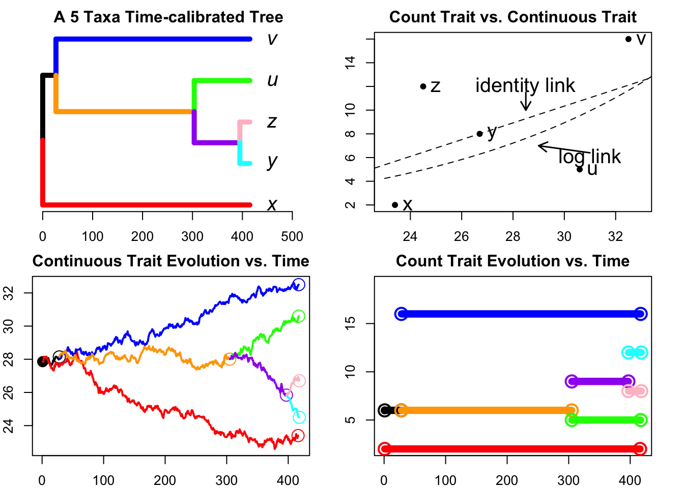
plot(phy,edge.width = 5,label.offset=0.05,cex=1.5,edge.color=colors22)
title("A 5 Taxa Time-calibrated Tree ")
axisPhylo(side=1,backward = FALSE)
plot(rawy~X,col="black",pch = 16,xlim=c(23,33),main="Count Trait vs. Continuous Trait",ylab="Count Trait",xlab="Continuous Trait")
XX=X+0.5
tiplab<-c("x","y","z","u","v")
for (i in 1:5){text(x=XX[i],y=rawy[i],tiplab[i],col="black",cex=1.5)}
ols<-lm(rawy~X)
abline(a=ols$coefficients[1],b=ols$coefficients[2],lwd=1,lty=2)
logols<-lm(log(rawy)~X)
curve(exp(logols$coefficients[1])*exp(logols$coefficients[2]*x),23,35,add=TRUE,col="black",lty=2)
text(x=31,y=6,"log link",col="black",cex=1.5)
arrows(31,6.4,29,7 ,lwd=1.5, length=0.1, code=2,col = "black")
text(x=28.5,y=12,"identity link",cex=1.5)
arrows(28.5,11.5,28.5,10 ,lwd=1.5, length=0.1, code=2)
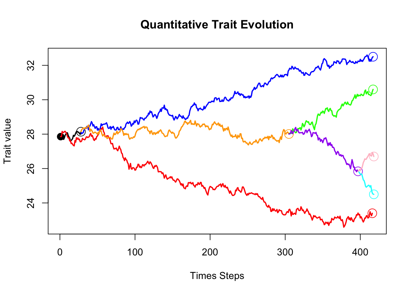
PlotTreeHistory(phy=phy,pathdata=bbpathdata,main="Continuous Trait Evolution vs. Time",colors=colors)
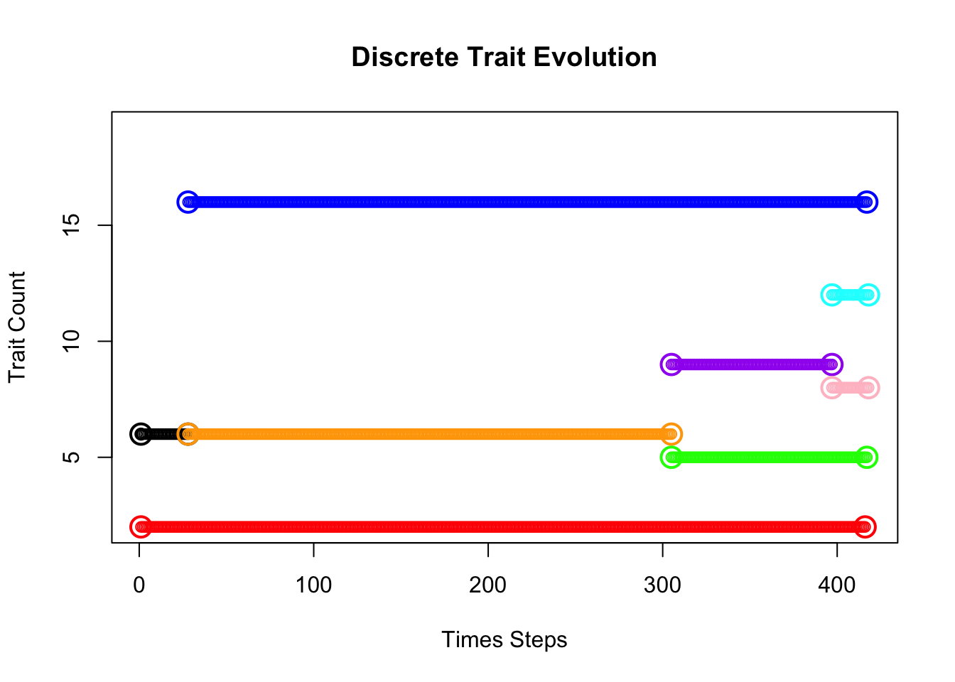
PlotTreeHistory.Discrete(phy=phy,pathdata=path.countdata,main="Count Trait Evolution vs. Time",colors=colors)