rm(list=ls())
library(MASS)
library(TreeSim)
set.seed(443)
size<-5
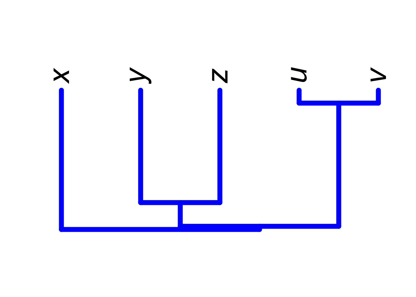
phy<-sim.bdtree(b=1, d=0, stop=c("taxa", "time"), n=size, t=4, seed=0, extinct=TRUE)
C<-vcv(phy)
X<-c(23.4,26.7,24.5,30.6,32.5)
rawy = c(2,8,12,5,16)
colors22<-c("cyan","pink","purple","green","orange","blue","red","black")
phy$tip.label<-c("x","y","z","u","v")
plot(phy,edge.width = 8,direction="upward",label.offset=0.05,lwd=3,cex=3,edge.color="blue")
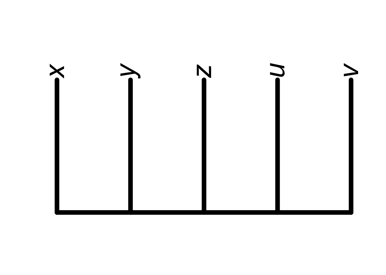
starphy<-stree(size)
starphy$tip.label<-c("x","y","z","u","v")
plot(starphy,edge.width = 8,direction="upward",label.offset=0.05,lwd=3,cex=3,edge.color="black")
############################
#### Regression with star tree ####
############################
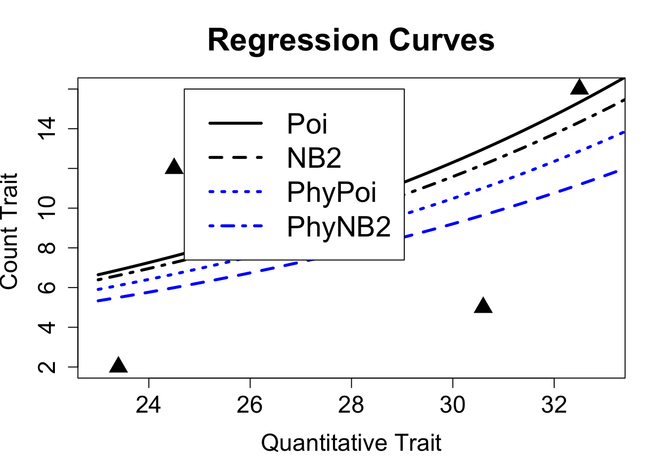
plot(rawy~X,col="black",pch = 17,xlim=c(23,33),cex=2,xlab="Quantitative Trait", ylab="Count Trait ", main="Regression Curves",cex.main=2,cex.lab=1.5,cex.axis=1.5)
fitnpoi <-glm(rawy~X,family = "poisson")
fitnb2<-glm(rawy~X,family = negative.binomial(theta = 10))
curve(exp(-0.130)*exp(0.088*x),23,35,add=TRUE,col="black",lwd=3,lty=1)
curve(exp(-0.100)*exp(0.085*x),23,35,add=TRUE,col="black",lwd=3,lty=4)
curve(exp(-0.120)*exp(0.078*x),23,35,add=TRUE,col="blue",lwd=3,lty=2)
curve(exp(-0.110)*exp(0.082*x),23,35,add=TRUE,col="blue",lwd=3,lty=3)
legend(24.7, 16, legend=c("Poi", "NB2", "PhyPoi", "PhyNB2"), col=c("black","black", "blue", "blue"), lty=c(1,2,3,4), cex=1.8,lwd=3)